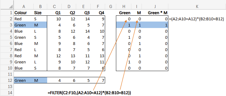
How FILTER handles multiple criteria

The structure I use all the time:
=FILTER(C2:F10, (A2:A10=A12) (B2:B10=B12))

In this example I filter for the following:
Colour = Green -> (A2:A10=A12)
Size = M -> (B2:B10=B12)

Each condition returns a vertical array:
(A2:A10=A12) -> {0;1;0;1;0;0;0;1;0}
(B2:B10=B12) -> {0;1;0;0;1;0;1;0;0}

Multiplying these arrays gives:
{0;1;0;0;0;0;0;0;0}

Excel treats TRUE/FALSE as 1/0 (Boolean logic), only rows where both conditions are TRUE (11 =1) are returned.

The FILTER formula returns an array of {4,6,5,7) from C2:F10 as the match for Green & M.

This is a small technique that unlocks the real power of dynamic arrays.
It's quick, dynamic and scales for mulitple criteria.